VIBES & BMW Group
Virtually optimizing and selecting the best components to reduce NVH issues can be carried out with Frequency Based Substructuring (FBS) using test data. Applying this method in the early development stage allows OEMs to bridge the gap between the concept phase and the first actual vehicle prototype. With the support of the Eurostars program, VIBES is developing software applications to implement FBS. This article presents a successful implementation of the method on an electric drivetrain. The entire project has been conducted in collaboration with BMW. The full paper can be found here.
The goal
The investigation aims to verify whether FBS can be used to accurately predict the NVH performance of an electric vehicle, taking into account the noise and vibrations produced by the electric drive unit. The results obtained using substructuring will be compared with validation measurements of the assembled system.
The component
The component analyzed is an electrical drivetrain. In the assembly, 3 subsystems can be distinguished: the EDU (Electric Drive Unit), the RAC (Rear Axle Carrier), and the TMB (the bodywork or “trimmed-body”). A total of 8 coupling points can be identified: 4 of them connect the EDU to the RAC, and the other 4 connect the latter to the trimmed body. The following figure shows the original full-vehicle assembly, for which operational run-up measurements have been conducted. In the figure, it is possible to see the three-stage FBS model: here the assembly is visualized as a chain of the 3 subsystems and the 8 coupling points.
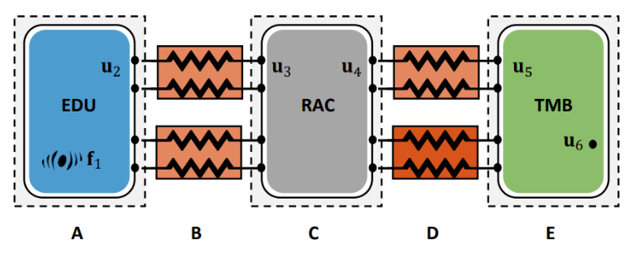
Schematic overview of the e-drivetrain assembly. Source: link
Technical approach
Overview
The dynamic behavior of each subsystem shown in the figure is experimentally obtained using the software DIRAC. The dynamic stiffness of the rubber mounts is calculated with the inverse substructuring method. The components are then coupled using the compliant FBS coupling technique. This is the case because the rubber bushings that connect the subsystems are made of flexible material with negligible mass.
The active excitations of the EDU are described with blocked forces, which are obtained using the so-called free velocity method. The blocked forces are later applied to the coupled system. The results of the FBS analysis are then compared with the measurements of the assembled system as validation.
Subsystems FRFs calculation
To create a full vehicle model using FBS, the dynamic behavior of each subsystem is needed. The model of each component has been obtained through impact testing in a free-free configuration. This means that all the components have been either freely suspended or placed on air springs to have the interface Degrees of Freedom (DoFs) free to displace.
The test-based models are obtained using DIRAC, which is designed to optimize the test-based modeling, ensuring high-quality results into the kHz range. The modeling process consists of 4 steps:
- Design of Experiment (DoE) preparation: in this step, the design of experiment is recreated in a 3D environment. The CAD geometries of the subsystems are loaded in DIRAC, and the sensors, excitations and Virtual Points (VPs) are defined.
- Instrumentation and DAQ setup: the accelerometers are attached to the components following the DoE previously created and are connected to the Müller-BBM MKII data acquisition system. Two impact hammers have been used, one with a rubber tip (to excite low frequencies) and one with a nylon tip (for higher frequencies), which are automatically merged in the software.
- Impact testing: following the predefined DoE, DIRAC guides the user in the measurement phase. Here, all the impacts are performed and the FRFs of the components are calculated. Multiple Virtual Point indicators are used to evaluate the quality of the measurements. Operational Deflection Shape animations (ODS) are used to verify the correct sensors’ orientations.
- Virtual Point Transformation (VPT) and analysis: the VPT is applied live during FRF measurement. The quality of the transformed FRFs is verified through other quality indicators implemented in DIRAC such as consistency, reciprocity and passivity of the resulting VPs.
An example of the VPT FRFs of the rear axle carrier in DIRAC is shown in the following figure.
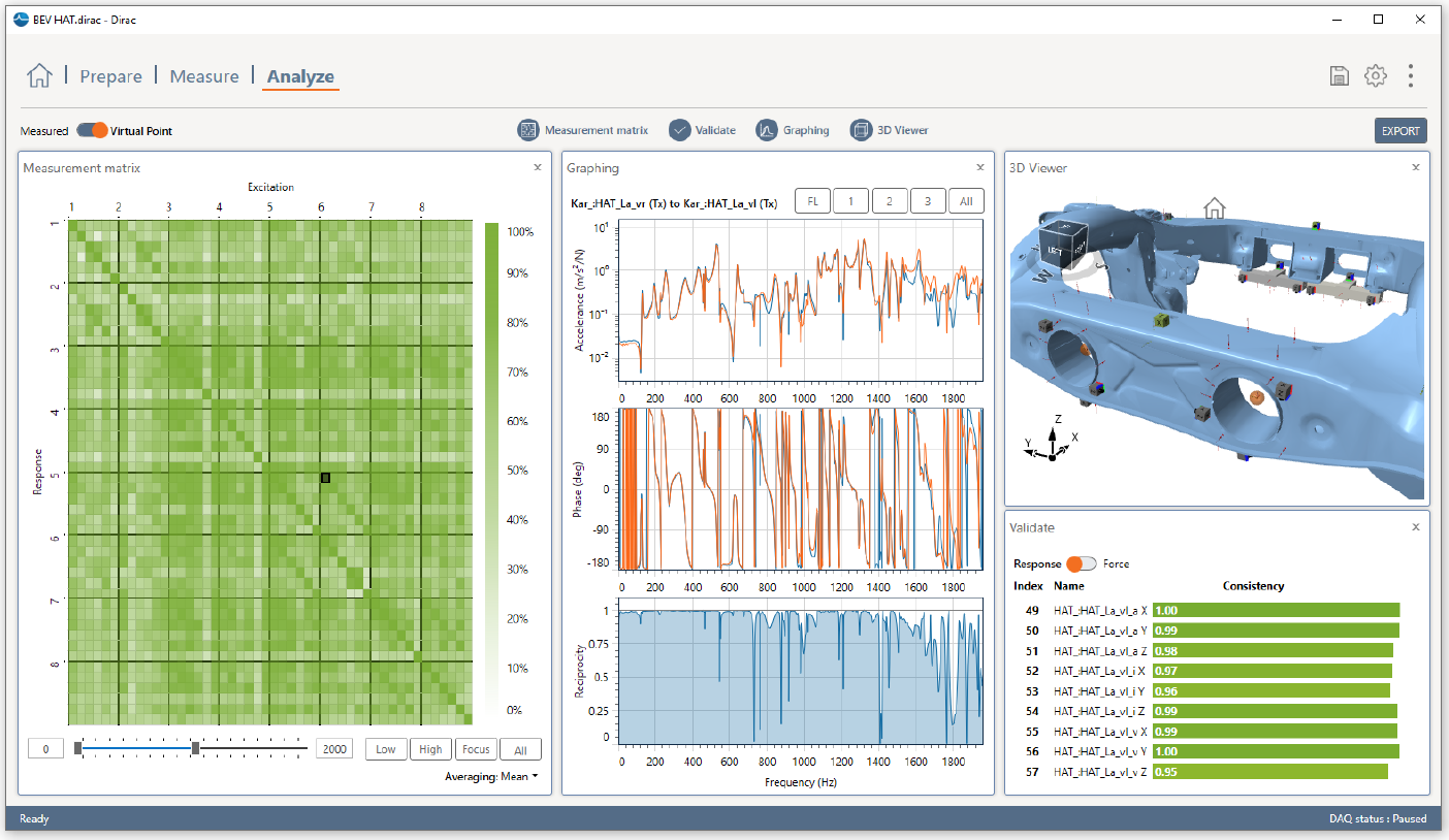
The Virtual Point FRF matrix of the 8 coupling points of the rear axle carrier.
The whole process has been applied to each of the subcomponents (EDU, RAC, and TMB), and their dynamic behavior is represented by respectively $$\mathbf{Y}^\mathrm{A}$$, $$\mathbf{Y}^\mathrm{C}$$ and $$\mathbf{Y}^\mathrm{E}$$ (notation from the first figure). In addition, to validate the substructuring of the first connection stage (obtained using FBS), a test-based model of the assembled EDU and RAC has been measured as well.
Each Virtual Point has been described with 6 DoFs (3 translations and 3 rotations).
Mount stiffness modeling
After obtaining the test-based models of the three subsystems, it is necessary to characterize the rubber bushings. A combination of DIRAC and the VIBES Toolbox for MATLAB is used for the mounts modeling.
Aluminum transmission simulators have been machined to fit tightly to the rubber bushing cylinder and its ends. A total of 14 triaxial accelerometers have been glued, and 37 impact positions and 2 Virtual Points (with 6 DoFs each) have been defined in DIRAC. The complete design of experiment made in DIRAC can be seen in the next figure.
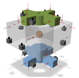
Model of the rubber bushing in DIRAC. Source: link
After impact testing, the 12×12 Virtual Points transformed matrix $$\mathbf{Y}_{\mathrm{qm}}(\omega)$$ is calculated and inverted to obtain $$\mathbf{Z}^{\mathrm{mnt}}(\omega)$$ which is the dynamic stiffness matrix of the assembly (mount and transmission simulators).
The inverse substructuring technique has proven that the off-diagonal blocks of the dynamic stiffness matrix approximate the dynamic stiffness of the mount only. This is valid up to the first internal resonance of the mount. The bushing stiffness obtained with the inverse substructuring method has been compared with the data provided by the mount supplier. From the following figure, it can be seen that the curves align well.
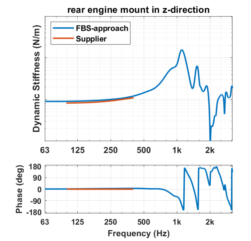
Comparison of bushing stiffness provided by the supplier and calculated with inverse substructuring. Source: link
The bushing stiffness obtained with inverse substructuring is later used when the components are coupled to obtain the substructured vehicle model.
Operational measurements and blocked forces calculation
Directly measuring the internal forces produced by the EDU is not possible. For this reason, a set of equivalent forces $$\mathbf{f}_2^{\mathrm{eq}}$$ (also called blocked forces $$\mathbf{f}_2^{\mathrm{bl}}$$) are used. They are an inherent property of the EDU itself (independent of the receiver). When applied at the interface of the assembled system, they produce on the passive side the same response that the internal forces would cause.
The blocked forces are obtained on the active side and are defined as
$$\mathbf{f}_2^{\mathrm{bl}} = \left ( \mathbf{Y}_{\mathrm{22}}^\mathrm{A} \right )^{-1} \mathbf{u}_2^{\mathrm{free}}$$
where $$\mathbf{Y}_{\mathrm{22}}^\mathrm{A}$$ is the dynamic stiffness of the drivetrain at the active side interface and $$\mathbf{u}_2^{\mathrm{free}}$$ are the operational accelerations. In addition, to validate the results at the end of the project, operational measurements of the engine attached to the full-vehicle are performed. For the purpose, sound pressure levels ($$\mathbf{u}_6^{\mathrm{val}}$$) at the passengers’ ears are recorded with microphones.
Components compliant coupling
The goal of the components’ coupling is to build the transfer functions of the full assembly using the FRFs of the three single components (EDU, RAC, and TMB). Rigid LM-FBS consists in assembling the dynamic matrices of the three subsystems ($$\mathbf{Y}^\mathrm{A}$$, $$\mathbf{Y}^\mathrm{C}$$ and $$\mathbf{Y}^\mathrm{E}$$) enforcing strict coordinate compatibility and force equilibrium for each matching DoF.
For this case, the main equation of LM-FBS is built up assembling the 3 matrices of the subsystems as follows:
$$\mathbf{Y}^\mathrm{coupl}_{\mathrm{rigid}} = \mathbf{Y} \left ( \mathbf{I} – \mathbf{B}^\mathrm{T} \left ( \mathbf{BYB^\mathrm{T}} \right )^{-1} \mathbf{BY} \right )$$
Where
$$ \mathbf{Y} \overset{\Delta}{=} \begin{bmatrix}
\begin{bmatrix}
\mathbf{Y}^\mathrm{A}_{11} & \mathbf{Y}^\mathrm{A}_{12}\\
\mathbf{Y}^\mathrm{A}_{21} & \mathbf{Y}^\mathrm{A}_{22}
\end{bmatrix} & \mathbf{0} & \mathbf{0}\\
\mathbf{0} & \begin{bmatrix}
\mathbf{Y}^\mathrm{C}_{33} & \mathbf{Y}^\mathrm{C}_{34}\\
\mathbf{Y}^\mathrm{C}_{43} & \mathbf{Y}^\mathrm{C}_{44}
\end{bmatrix} & \mathbf{0}\\
\mathbf{0} & \mathbf{0} & \begin{bmatrix}
\mathbf{Y}^\mathrm{E}_{55} & \mathbf{Y}^\mathrm{E}_{56}\\
\mathbf{Y}^\mathrm{E}_{65} & \mathbf{Y}^\mathrm{E}_{66}
\end{bmatrix}
\end{bmatrix} $$
And B is the Boolean compatibility matrix:
$$\mathbf{B} \overset{\Delta}{=} \left [ \begin{bmatrix}
\mathbf{0} & \mathbf{I}\\
\mathbf{0} & \mathbf{0}
\end{bmatrix} \begin{bmatrix}
\mathbf{-I} & \mathbf{0}\\
\mathbf{0} & \mathbf{I}
\end{bmatrix} \begin{bmatrix}
\mathbf{0} & \mathbf{0} \\
\mathbf{-I} & \mathbf{0}
\end{bmatrix} \right ]$$
In the current case, however, the three subsystems are connected through flexible rubber bushing, and therefore, the compliant coupling technique could be the best technique to use. This fact has been investigated comparing the FRFs of the components at the engine side and after the bushing, as shown in the following figure.
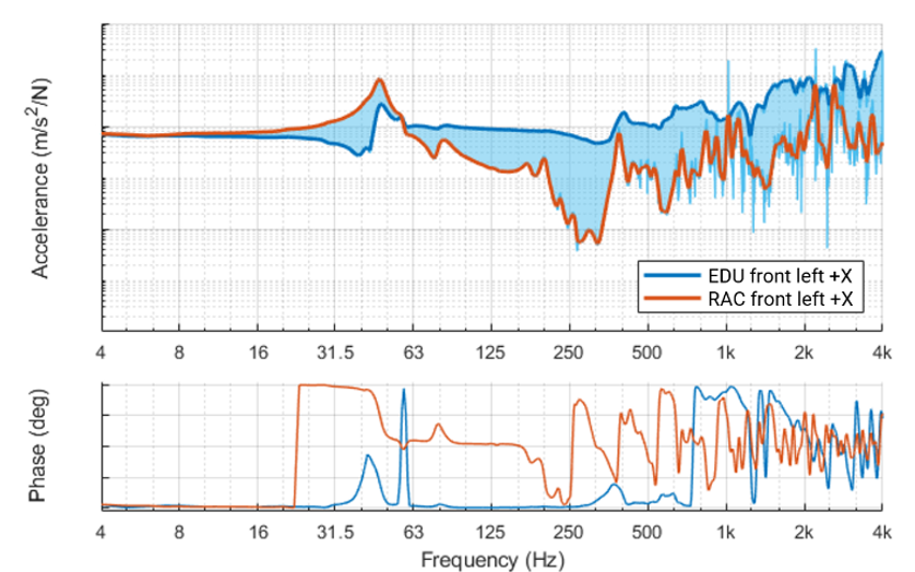
FRFs of the EDU and RAC before and after the bushing.
It can be observed that up to about 16 Hz, the EDU and RAC transfer functions overlap, which means that the two components and the mount behave as a rigid body. After that frequency level, the curves start deviating one from the other, and the flexibility of the rubber bushing starts playing a role.
This deviation of the dynamic behavior between the EDU and the RAC can also be noticed when observing the two components’ Operational Deflection Shape (ODS). The next figure shows two snapshots of the ODS at a frequency of 40 Hz. It can be noticed that a relative movement between the two components is present at this frequency.
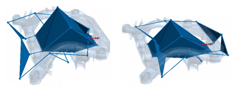
Snapshots of the operational deflection shape of the EDU and the RAC at 40 Hz.
This analysis proves that compliant coupling is the coupling technique that needs to be used for the current case. The calculated dynamic stiffness of the rubber bushings is taken into account at the relevant coupling DoFs. For this reason, the formula used for the compliant coupling considers the calculated dynamic stiffness of the bushings ($$\mathbf{Y}^\mathrm{mnt}$$):
$$\mathbf{Y}^\mathrm{coupl}_{\mathrm{compliant}} = \mathbf{Y}\left ( \mathbf{I}-\mathbf{B}^\mathrm{T} \left ( \mathbf{BYB}^\mathrm{T} + \mathbf{Y}^\mathrm{mnt} \right )^{-1} \mathbf{BY}\right )$$
The compliant LM-FBS coupling for this application has been performed in the VIBES Toolbox for MATLAB.
Subsystems coupling and first stage validation
To verify the accuracy of the substructured model, the FRFs of the coupled EDU and RAC $$(\mathbf{Y}^\mathrm{A + B+C})$$ are compared with the data of the assembled EDU and RAC that have been previously measured with DIRAC. The results can be seen in the next figure. Here, the accelerance and phase of the FRFs at the engine side (left) and after the bushing (right) are shown.
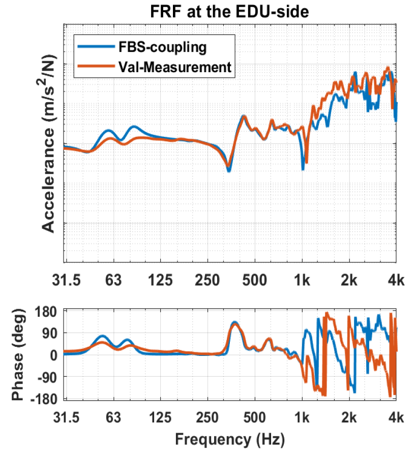
FRF comparison of an excitation at the engine in Z-direction to the rear-right engine measurement point in Z-direction.
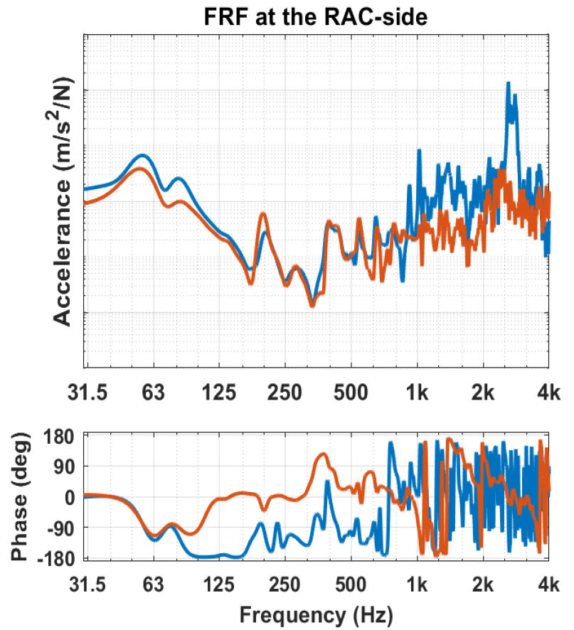
FRF comparison of an excitation at the engine in Z-direction to the rear axle carrier after the mount in Z-direction.
Validation of the coupling of the drive unit with the rear axle carrier. Source: link
Looking at the left figure, it can be noticed that the two curves overlap quite well up to 1 kHz. Also after the mount (right figure) the two curves match, but deviations at higher frequencies are present. The cause of the mismatch could be either minor positioning errors in the measurements or some numerical effects during coupling.
It can be concluded that the compliant coupling with the simplified bushing models performs well in the current situation.
After validating the engine’s coupling with the rear axle, the last subsystem (trimmed body) is added. At this stage, the substructured full vehicle model ($$\mathbf{Y}^\mathrm{full \; vehicle}$$) is available.
Component-based TPA / Applying the excitations to the substructured model
In the next step, the blocked forces are applied to the full-vehicle model that has been built using FBS ($$\mathbf{Y}^\mathrm{full \; vehicle}$$ ) and the resulting sound pressures at the microphones placed at the passengers’ ears locations ($$\mathbf{u}_6$$) are calculated using the formula
$$\mathbf{u}_6 = (\mathbf{Y}^\mathrm{full \; vehicle}) \mathbf{f}_2^{\mathrm{bl}}$$
The results are compared with the validation measurements performed with the engine attached to the full-vehicle ($$\mathbf{u}_6^{\mathrm{val}}$$). The following figures show respectively the Campbell diagram of the measured sound pressure levels and the predicted ones at the passengers’ ears.
The two plots show a good match between measurements and predictions up to 500 Hz. At about 850-900 Hz, the model obtained through component TPA and substructuring presents a mismatch in the coupled FRFs. Overall, the two diagrams show the same pattern except for the mismatch.
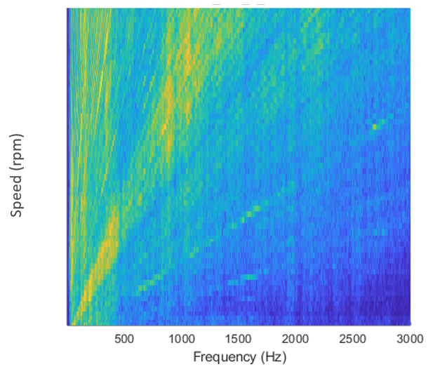
Measured sound pressure level.
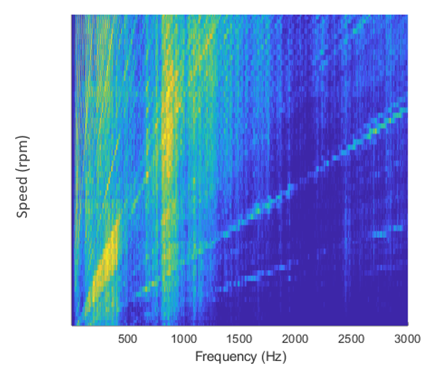
Predicted sound pressure level using component TPA and the substructured full vehicle model.
Campbell diagrams of the measured and predicted sound pressure levels at the microphone’s positioned at the passengers’ ears.
It can be concluded that the full vehicle model built with frequency based substructuring performed well in the component TPA carried out in this project.
Benefits of FBS
This project proved that FBS is an excellent solution to obtain full vehicle models starting from single components. It has also been demonstrated that the dynamic stiffness of rubber bushings calculated through inverse substructuring matches with the mounts data provided by the suppliers.
The benefits of using FBS are listed:
- FBS allows for the combination of subsystem models that get assembled to form a full vehicle model.
- With FBS, it is possible to exchange substructures and directly simulate the dynamics of the new system leaving all the other subsystems unchanged.
- The subsystems dynamics can either originate from Finite Element Models (FEM) or from component or subsystem measurements, allowing for a hybrid development approach.
- The full-vehicle model, simulated through FBS, can be used to close the gap in full-vehicle analysis and responsibility between the early-stage conception phase and the first actual prototype in hardware.
- Subsystems FRFs/NTFs are typically obtained at higher signal-to-noise ratios (SNR) than full-vehicle FRFs/NTFs, and thus a better overall quality can be reached.
Acknowledgment
The shown methods of frequency based substructuring and mount stiffness characterization with inverse substructuring were applied and validated within the scope of a project with industry partner BMW. VIBES likes to thank our partner for providing the opportunity to apply and prove our methodology and to publish the results within a case study.
Do you want to know more? Get in touch with VIBES or read more cases, using the buttons below! You can also download the full paper here!
More information
Maarten van der Seijs
Head of Technology
Maarten is responsible for the technology within VIBES. He co-founded VIBES after doing his PhD research at BMW in Munich.
Eleonora Cesari
Business Developer
Eleonora holds a MSc. in Aerospace Engineering. After gaining experience at Audi and Daimler, she joined VIBES to improve our sales.