VIBES & Hyundai Motor Company
Road noise has known to be one the major noise sources in a modern car. While drivetrain noise levels nowadays go down considerably – already due to replacement of the combustion engine by an electric one – noise induced by the tire-road contact remains an important NVH aspect. For a typical consumer car, the structure-borne noise contribution sits predominantly in the frequency range from 20-500 Hz, whereafter the airborne contributions gradually take over. Within this bandwidth, one sometimes speaks of “booming” noise between approximately 20-200 Hz, a smaller band associated with the tire cavity typically around 200-250 Hz and “rumble” noise up to 500 Hz. Mitigating road noise means reducing the vibration propagation from the tire-road contact to the driver’s and passengers’ ears. A major point of focus for an OEM is the suspension subsystem, which comprises the knuckle-wheelhub assembly, the spring/damper and the various linkages that defines the suspension mechanism. The figure below shows a schematical depiction of a typical rear suspension system.
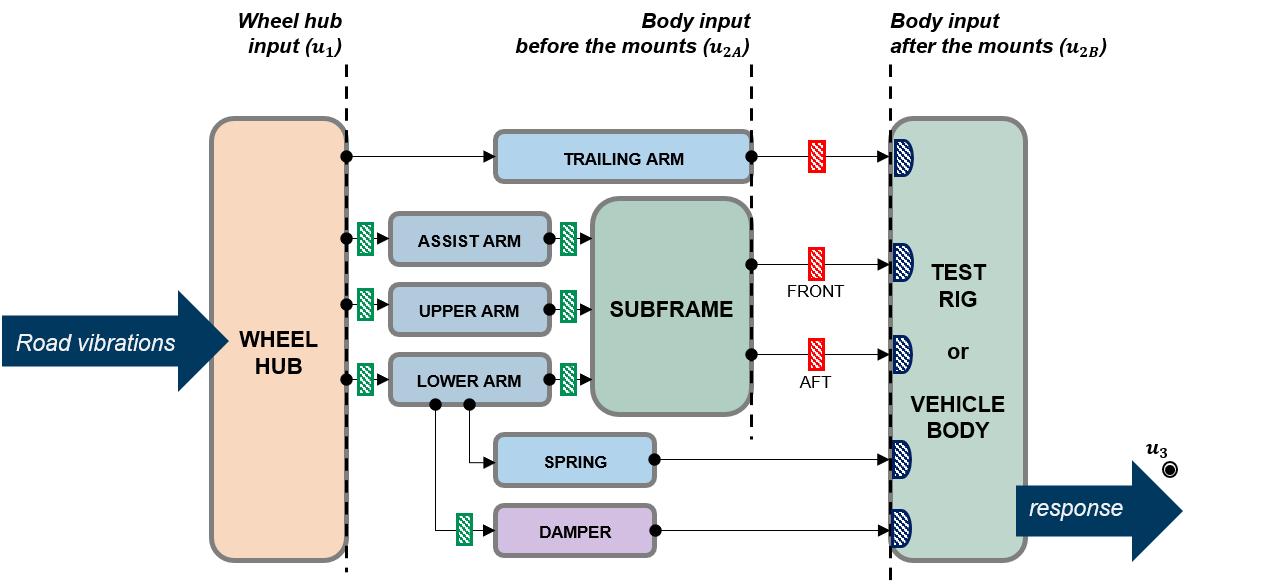
Schematic overview of the rear wheel supension system for a single side
Many of the suspension linkages are interconnected by rubber bushings. Each of those bushings is designed carefully for optimal performance, considering different aspects such as handling, drive comfort and of course NVH performance. In this design, one often finds trade-offs between the mentioned aspects, which limit the design space to certain dynamic stiffness ranges in the axial and radial directions of the bushing. As usual in dynamics, changes to particular bushings affect the transmission of road noise more than others. The optimization of the suspension for NVH performance is therefore a multi-variable challenge and needs a process that is able to evaluate changes on the full-vehicle level.
In this paper we describe a process that uses measurements on a rear-wheel suspension test bench, vehicle noise transfer functions and a state-of-art approach using virtual points to ensure compatibility of the two setups. Essentially, we demonstrate application of Component-based TPA , using several approaches to estimate the blocked forces.
The full paper is published on Researchgate.
Approach
The Component TPA approach with use of virtual points allows for a unified TPA simulation procedure. The blocked forces $$ \mathbf{f}^\textrm{bl}_2 $$ will be applied to the full-vehicle transfer functions $$ \mathbf{Y}^\textrm{AB}_{32} $$ to predict the driver’s ear responses $$\mathbf{u}_3$$ in the vehicle:
$$ \mathbf{u}_3 = \mathbf{Y}^\textrm{AB}_{32} \mathbf{f}^\textrm{bl}_2 $$
Because of the presence of rubber bushings, it is relevant to consider the point of application of blocked forces in terms of before and after the mounts, namely:
1. After the mounts ($$ \mathbf{f}^\textrm{bl}_{2B} $$): blocked forces include the effects of the bushings to the bodywork. The forces can be applied straight-away to the full vehicle bodywork on the passive side;
2. Before the mounts ($$ \mathbf{f}^\textrm{bl}_{2A} $$): blocked forces do not include the effect of the bushings. This allows changing the bushings by virtually adjusting the FRF of the full vehicle and applying the blocked forces to this FRF on the active side.
In this study, both variants are considered. The configuration using passive-side blocked forces after the mounts is used as the base case, as it aligns with the rigid rig configuration.
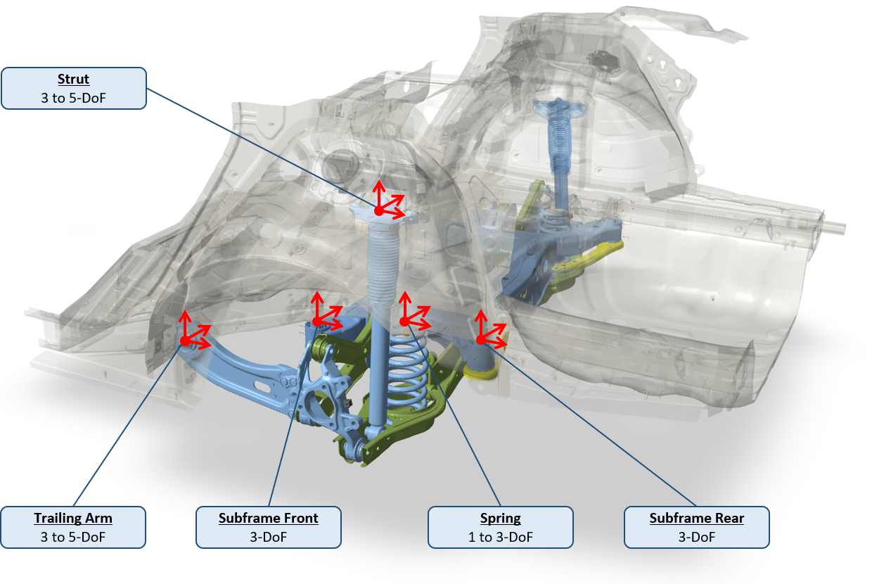
The 5 connection points of the rear suspension and their modeling strategy using virtual points
Connection points
In this study we used virtual points at prescribed locations to have a common interface between all test assemblies. The figure above shows the 5 connection points of the rear suspension to the vehicle bodywork: the trailing arm, subframe front and rear mounts, the strut with damper and the spring. In total, we consider the 10 coupling points for the left and right side simultaneously.
As indicated, the modeling strategy can be chosen for each coupling point differently. The four subframe mounts typically only exhibit translational motion and can be well described by 3-DoF translational dynamics. For the trailing arm and the strut, additional rotational DoF have been added for optional moment information. This was also done to match the instrumentation of the force sensors on the test bench: for these points two sensors per coupling point were used which allow estimation of two additional moments.
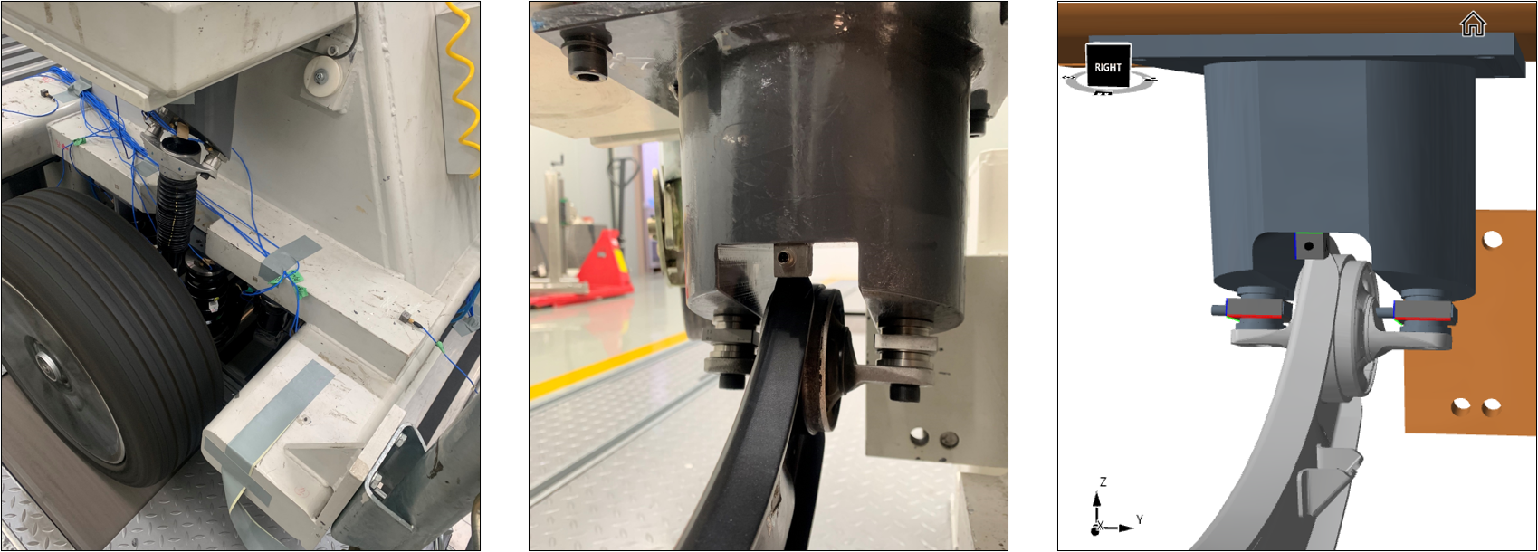
The rigid test rig. Left: the tire on the dyno. Center: two force gauges installed at the trailing arm passive side connection point. Right: the same setup in the DIRAC modeling environment showing the location of the force gauges.
Rigid rig
The rigid test rig has been used and described in previous studies. The rig is optimized for direct force measurement and has force gauges installed at the connecting points to the body after the bushings; see the figure above. The measured forces can thus be interpreted as direct blocked forces after the mount, or $$ \mathbf{f}^\textrm{bl}_{2B} $$ in notation of the TPA Framework. Although this is theoretically correct, successful application warrants consideration of some important practical aspects:
Processing of the force gauge data. The force gauges are installed in the most practical locations, namely between the rigid rig adapters and the bushings and along the direction of the bolts that normally connect the suspension to the vehicle. This means that every coupling point has a somewhat local coordinate frame, that may be cumbersome to match with any transfer function measured on the vehicle. The virtual point approach is therefore used to transform all measured operational forces into the global coordinate frame, as well as to sum them in a kinematically correct manner. In this case of measured forces, we use the transpose of the IDM matrix for the force gauges $$\mathbf{g}_{2B}$$ to the virtual points:
$$ \mathbf{f}^\textrm{bl}_2 = \left( \mathbf{R}_\textrm{f} \right)^T \mathbf{g}^\textrm{oper}_\textrm{2B} $$
The IDM matrix is automatically computed using DIRAC for the design of experiment, as shown in the figure above.
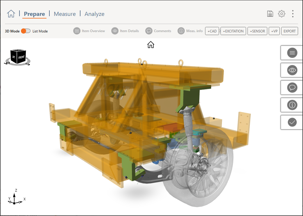
The soft rig setup in DIRAC. The flexible adapters are shown in green.
Rigidness of the test rig. Direct blocked force measurement is known to be most effective for low frequencies. The validity of the rigid boundary assumption breaks down with increasing frequencies, due to flexibility of the test rig. As shown in the figure of the rigid test rig, the rigid rig adapters are optimized for maximum stiffness, being constructed from solid steel. Nevertheless, the first eigenmodes of the test rig may have a degrading effect on the blocked forces.
Soft rig
One of the focus points of the study was to also investigate an approach using more flexible test rig adapters. The resulting “soft rig” construction is shown in the figure above. In this case, accelerometers at the passive side of the connection points are used to calculate blocked forces at the passive side in a matrix-inverse way; a method known as in-situ characterization. A great benefit is now that both blocked forces before and after the mount can be computed with the same ease. Both cases use the same passive-side indicator responses; the difference lies in the virtual point forces of the FRF matrix to invert.
Active-side:
Passive-side:
$$ \mathbf{f}^\textrm{bl}_{2A} = \left( \mathbf{Y} ^\textrm{AR}_\textrm{42A}\right)^+ \mathbf{u}_4 $$
$$ \mathbf{f}^\textrm{bl}_{2B} = \left( \mathbf{Y} ^\textrm{AR}_\textrm{42B}\right)^+ \mathbf{u}_4 $$
The FRF matrices with virtual point force columns have been created using DIRAC. These are sometimes called “right-sided” virtual point FRF matrices, as the virtual point transformation is only applied to the FRF columns, which is sufficient for in-situ calculation. The overdetermination of the matrix inversion is kept at 150-200%.
Vehicle
FRF and operational tests have also been conducted on the full vehicle. Full-vehicle FRFs were obtained similar as for the compliant test rig, namely for impact points before and after the mounts to the bodywork and again transformed to virtual points. These virtual point forces are now directly compatible with the virtual point blocked forces coming from the test rigs, as they are both defined in the unique coordinate frame of the virtual points.
The FRF tests have again been conducted using DIRAC, connected to a Müller-BBM PAK MK2 system for acquisition of about 200 channels, including some microphones at the ear positions. In order to excite the full bandwidth of 0-500 Hz, two impact hammers have been used with different qualities: a heavier PCB 086D05 hammer with rubber tip to cover the low frequencies (0-200 Hz) with sufficient energy, and a lighter PCB 086C03 hammer with nylon tip to excite up to several kHz.
DIRAC low- and high-pass filters the data correspondingly and makes sure that the measurement data is correctly added in the estimation of the transfer functions. The result is near-perfect coherence and signal-to-noise for all FRF functions in the frequency range of interest. This is illustrated in the figure below.
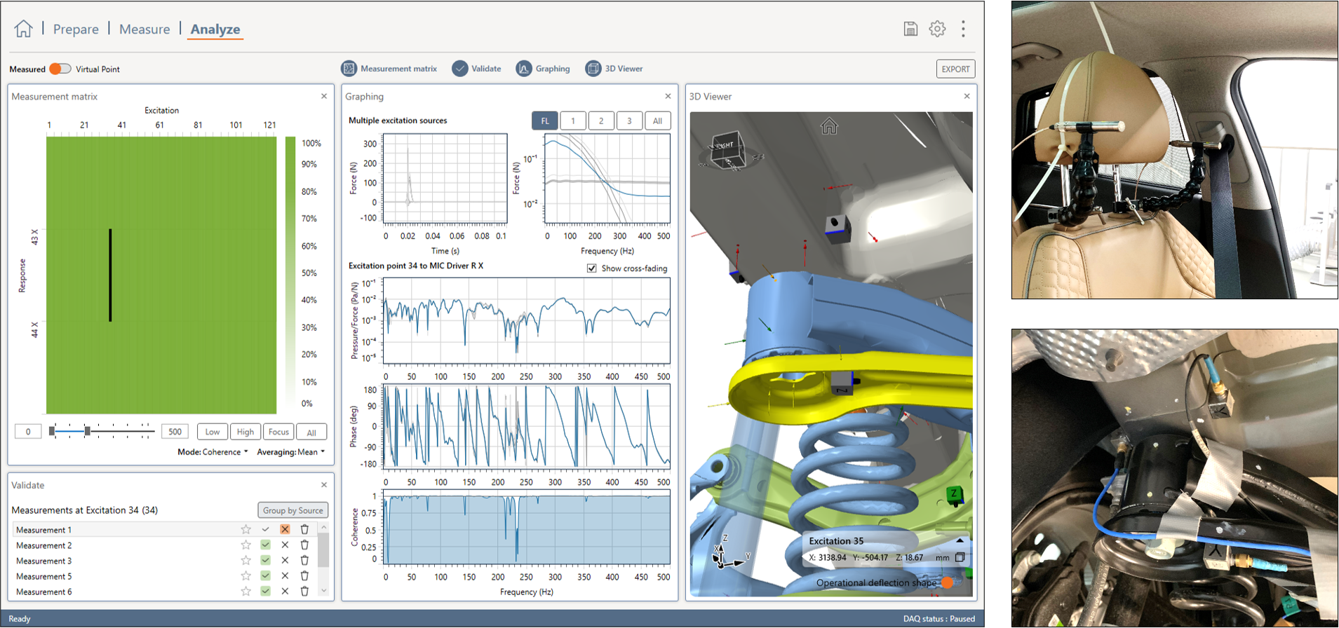
Full vehicle FRF measurement in DIRAC. Two impact hammers were used to properly excite the full frequency range of 0 500Hz; their data (grey is merged directly in the estimation of the transfer functions (blue curve).
Results
Let us now discuss the application of the methods described above. The operational cycle used is for all test assemblies a run-up of the rear wheels on a dyno from 20 – 120 km/h. The recorded time data is converted to 1-second blocks with 50% overlap and Hann-windowed before computed into frequency spectra. Whereas DIRAC is used for acquisition and virtual point transformation of all FRFs, all processing and TPA simulation is performed using SOURCE.
Rigid rig: direct blocked forces
Let us first look at the application of the direct blocked forces from the rigid test rig. In this case, the direct forces are obtained after the mounts, so are multiplied with the vehicle FRFs on the passive side. The figure below shows the simulation at the left driver ear compared to the direct measurement as a Campbell diagram, at the same color scale. It is clear to see that all relevant noise phenomena in the car are well represented by the test rig blocked forces applied to the vehicle noise transfer functions.
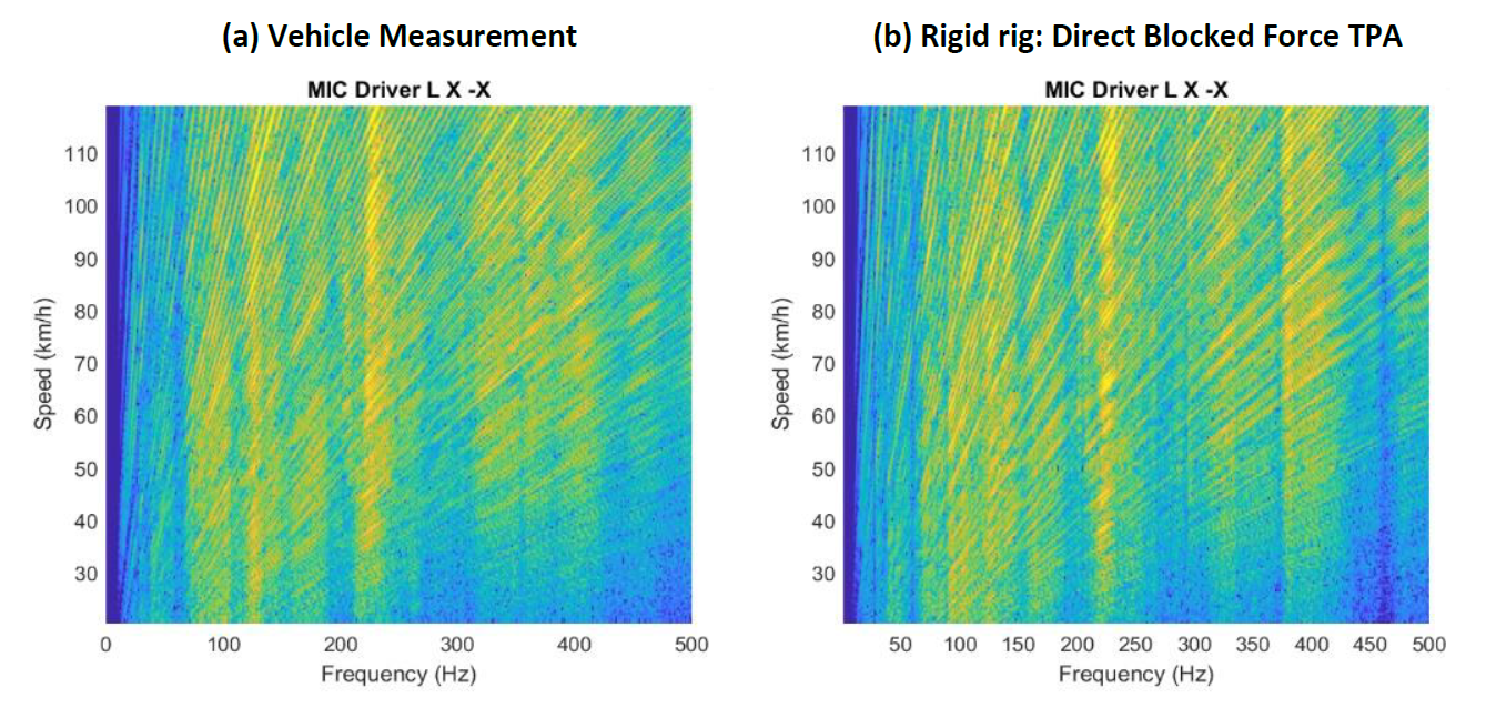
Validation measurement (a) compared to the prediction (b) of the direct blocked forces from the rigid rig.
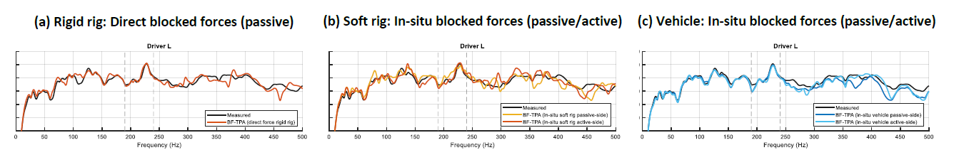
Result of blocked force application as dB(A) spectra. (a) rigid rig direct blocked forces. (b) Soft rig in-situ passive (yellow) and active (red) side. (c) vehicle in-situ passive (blue) and passive (cyan) side.
Another way of comparing the component TPA prediction with the measurement is by looking at the time-averaged spectra of driver-ear sound pressure levels in dB(A) over the full run-up from 20-120 km/h. The result of the rigid rig direct blocked forces is shown in the above figure (a) in red, where comparison is made with the vehicle measurement for a similar run up (black). The horizontal grid lines represent intervals of 10 dB(A). There is clearly a very high agreement, which demonstrates the power and simplicity of direct blocked force TPA through virtual points.
Soft rig: in-situ blocked forces
For the soft rig application, two cases are shown in the above figure (b): passive-side blocked forces (yellow) and active-side blocked forces (red). The passive-side blocked forces are indeed a result of VP-transformed impact points on the adapter blocks, whereas the active-side impacts are all applied on the suspension parts close to the mounts. The same indicator sensors were used for both calculations, namely all on the passive side. The matrix-inverse calculation has been calibrated by choosing the amount of singular values based on the number of active DoF in the inverse problem, using independent control points for validation.
Both predictions from the soft rig in-situ blocked forces show a good match well the general trend of the vehicle measurement. Compared with the direct force application, the curves tend to wobble a bit more. This is most likely explained by the sensitivity to (anti-)resonances in the soft rig FRFs, which plays a major role as it is inverted in the blocked force calculation. A benefit
over the direct blocked force approach is the availability of blocked forces before the bushings. These can be used in conjunction with vehicle FRFs where now the bushing stiffness can be altered by dynamic substructuring, leading to physically correct simulation of bushing changes.
Vehicle: in-situ blocked forces
Finally we present a similar in-situ approach for blocked forces calculated from the vehicle run-up. This can be seen as the true in-situ approach: the full vehicle on the dyno is the only test assembly under consideration. The prediction is shown in the figure above (c) for passive-side blocked forces (blue) and active-side blocked forces (cyan). The match up to 250 Hz is close to perfect for
both cases; higher up the agreement is also good. The active- and passive-side blocked forces show similar performance.
Conclusions
Several methods for blocked force characterization and component-based TPA have been discussed for the application of road noise NVH. A workflow has been described that uses virtual points to establish compatibility between two test rig setups for the suspension system and the full vehicle. It has been demonstrated that test rig measurements can indeed be used for accurate
prediction of NVH levels in the vehicle. The direct blocked force method has shown to produce good results, proving the rigidness of the test rig to be sufficient in the frequency range of interest. The in-situ methods using acceleration measurement and matrix inversion allow forces to be determined before or after the mount, both from test rig and vehicle measurements.
More info
Do you want to know more? Get in touch with VIBES or read more cases, using the buttons below! You can also download the full paper here!
More information
Maarten van der Seijs
Head of Technology
Maarten holds a PhD degree from the TU Delft on dynamic substructuring and as such is responsible for the technology within VIBES. Maarten co-founded VIBES when he came back to Delft from BMW in Munich, where he did his PhD research.